July 2019
(Note: all the previous SPC Knowledge Base in the measurement systems analysis category are listed on the right-hand side. Select this link for information on the SPC for Excel software.)

The experimental process is essentially the same. You have one or more operators. Each operator measures the same part(s) multiple times. The difference is that EMP immediately places the results on a control chart to assess how consistent, reproducible , and repeatable the measurement system is before moving forward with the characterization (calculations) of the various statistics, like the measurement error.
This month’s publication provides an overview of the techniques in EMP. In this issue:
- Introduction to EMP
- Relationship of Variances
- Consistency Study
- Short EMP Study
- Basic EMP Study
- Summary
- SPC for Excel Version 6 is Now Available!
- Quick Links
Please feel free to leave a comment at the end of this publication. You can also download a copy of this publication at this link.
Introduction to EMP
The EMP techniques are designed to help you answer questions you should have about your measurement system. Some of the questions from Dr. Wheeler’s book, EMP III: Evaluating the Measurement Process and Using Imperfect Data, are:
- Is the measurement system consistent over time?
- What is the precision of the measurement system?
- How many decimal places should be recorded?
- What is the resolution of the measurement system?
- Does the measurement system contain bias?
- How useful is the measurement system in characterizing the product?
- How much of the variation in the product measurements are due to the measurement system?
- Can the measurement system detect changes in the process?
It should be noted that the other measurement systems evaluation methods rely on question number 7 to determine if a measurement system is “good.” The value for the % of the total variance due to the measurement system is taken and compared to an arbitrarily set standard. So much information is missed with this approach.
The EMP techniques involve the use of control charts to ensure that your data are “valid” before any other calculations are done. The individuals control chart is used with the Consistency Study while the X-R control charts are used with the Short EMP Study and the Basic EMP Study. Each of these three studies is described below. Each has a previous SPC Knowledge Base article written that explains the technique in more detail. The table below shows what each technique can generate.
| EMPTECHNIQUE | OPERATORS | PARTS | PURPOSE |
|---|---|---|---|
| Consistency Study | 1 | 1 |
|
| Short EMP Study | 1 | Multiple |
|
| Basic EMP Study | Multiple | Multiple |
|
An overview of the three are given below. We will start, however, with a reminder of the relationship between the total variance, product variance and measurement error variance.
Relationship of Variances
You take a sample from your process. You test that sample using your measurement system. You get a result (X1). You take another sample and test that sample. You get another result (X2). Usually X1 does not equal X2. What are in these results? Two major components are present in each result: the variation in the product itself and the variation in the measurement system.
The basic equation describing the relationship between these variances is given below.
σx2= σp2+ σe2
where σx2= total variance of the product measurements, σp2= the variance of the product, and σe2= the variance of the measurement system.
The Consistency Study
A Consistency Study is run by having one operator measure the same part multiple times. The results are then placed on an individuals (X-mR) control chart. The control chart must be in statistical control before proceeding. If it is not, the measurement system cannot really measure anything until the reasons for the out of control points are found and corrected. Once the measurement system is consistent, you can move forward with the characterization of the measurement system (e.g., calculating the measurement error and bias).
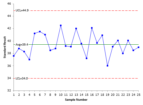
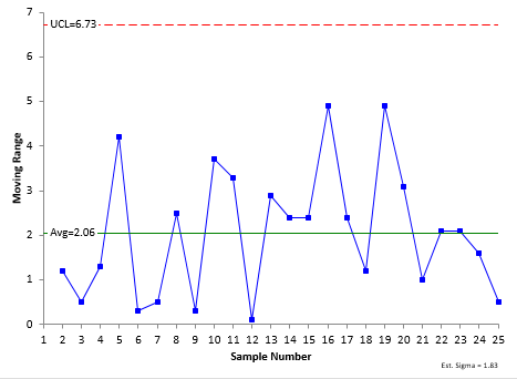
An example of a Consistency Study is given in our SPC Knowledge Base article, Evaluating the Measurement Process – Part 1. In this example, a viscosity standard is measured repeatably by one operator. The resulting control charts are shown below. The data are in the article.
Figure 1: X Chart for Repeated Viscosity Measurements for the Standard
Figure 2: Moving Range Chart for Repeated Viscosity Measurements for the Standard
Both charts are in statistical control. This means that the measurement system is consistent. Because the measurement system is consistent, you can begin to answer some important questions about your measurement system.
Do I Have Enough Data?
It is recommended that you have at least 10 degrees of freedom for a consistency study. This corresponds to 17 sample results. This example has 25 samples and 15.0 degrees of freedom. So, you have enough data. If not, you need to collect more data. Dr. Wheeler’s book contains tables to determine the degrees of freedom.
Is there Bias Present?
You can check for bias if a known standard was used. You do this by constructing a confidence limit around the average using the t-distribution. Two intervals are created: one for 90% and one for 99%. If the value of the known standard falls within the 90% confidence limit, there is no bias present. If it falls outside the 99% confidence interval, then there is detectable bias present. If it falls between the 90% and 99% confidence interval, there is potential bias present.
Is the Data Chunky?
This tells you if the measurement results on the same part/standard are rounded excessively. If there is excessive rounding, the data are considered chunky. Our publication, Chunky Data and Control Charts, explains this in more detail. The moving range chart is key here. The following is the test:
For X-mR charts: the data is chunky if the range chart has three or fewer possible values below the upper control limit.
As can be seen in Figure 2, there are more than three possible values, so the data are not chunky.
What is the Repeatability of the Measurement System?
This is usually given as a standard deviation using the average moving range:
σe= (mR)/1.128 =2.06/1.128 =1.83
where 1.128 is a constant based on the moving range of two.
Is the Measurement Increment Adequate?
The raw data used for the control charts above were measured to the nearest 0.1. This is the measurement increment. There is a statistic called the probable error (PE). It is given by 0.675σ_e.
PE = .675(σe) = .675(1.83) = 1.235
Half the repeated measurements will fall between the average and ± PE. PE can also be used to determine if the measurement increment is adequate. The resolution (measurement increment) should be between 0.2(PE) and 2(PE). That range for this example is 0.2471 to 2.471. The measurement increment is 0.1, which is outside this range. The data should be rounded to the nearest 0.2 and the analysis repeated. We will skip that part here. Please see our article, Probable Error and Your Measurement System, for more information.
How Much of the Total Variance is due to the Measurement System?
This is the characteristic that most people pay attention to. Remember the equation above: σx2= σp2 + σe2. The estimate of σe2 is known already. An estimate of the total variance (σx2) is needed. The best place to get this is from a range chart kept on the product viscosity. Suppose we have done that and the process sigma from the range chart is 2.76. We can then determine the % of the total variance that is due to the measurement system:
Total Variance due to Measurement System=(σe2/(σx2) = 1.832/2.762= 0.44=44%
How “Good” is My Measurement System?
This single value of the total variance due to the measurement system is what most people use to determine if the measurement system is good enough. For example, if the value is between 1% and 9%, AIAG says the measurement system may be acceptable for some situations. If it is greater than 9% (like this example), it is unacceptable. Dr. Wheeler has fundamentally changed how to look at how “good” a measurement system is. Dr. Wheeler based part of his rating on the value of the Intraclass Correlation Coefficient (ρ). This fancy name is simply the total variance due to the product itself (σp2).
ρ=σp2=1-(σe2/(σx2)= 1-1.832/2.762= 0.56=56%
The table below shows Dr. Wheeler’s system. It classifies a measurement system as a First Class, Second Class, Third Class or Fourth Class based on the value of ρ.
| Intraclass coefficient | Type of Monitor | Reduction of Process Signal | Chance of Detecting ± 3 Std. Error Shift | Ability to Track Process Improvements |
|---|---|---|---|---|
| 0.8 to 1.0 | First Class | Less than 10% | More than 99% with Rule 1 | Up to Cp80 |
| 0.5 to 0.8 | Second Class | From 10% to 30% | More than 88% with Rule 1 | Up to Cp50 |
| 0.2 to 0.5 | Third Class | From 30% to 55% | More than 91% with Rules 1, 2, 3 and 4 | Up to Cp20 |
| 0.0 to 0.2 | Fourth Class | More than 55% | Rapidly Vanishing | Unable to Track |
The table above answers three additional questions:
- How much the measurement system reduces the strength of a signal (out of control point) on a control chart.
- The chance of the measurement system detecting a large shift.
- The ability of the measurement system to track process improvements.
So, in this example, we have a Second Class monitor that will produce a reduction of signal from 10 to 30%, will be able to detect a large shift 88% of the time and track improvement up to Cp50. That is quite a bit for a measurement system that AIAG’s rating system would say is unacceptable. For more information on this classification system, please see our SPC Knowledge Base articles, Evaluating the Measurement Process – Part 1 and Acceptance Criteria for MSA. These articles provide a more detailed explanation of the classification system.
How Does the Measurement Error Impact Specifications?
Suppose you measure a part, and it is right below the upper specification limit. Is it within specification? Maybe or maybe not. The probable error defined above can help determine the probability that it is within specifications. You can use the probable error to determine manufacturing specifications. For example, with 96% manufacturing specifications, there is a 96% probability that an item with a measured value that falls between the manufacturing LSL and manufacturing USL conforms to specifications. The 96% manufacturing specifications are created by moving the customer specifications in by 2 probable errors. You can do this calculation for different probabilities. For more information on setting manufacturing specifications, please see our article, Specifications and Measurement Error.
Short EMP Study
A Short EMP Study is run by having one operator measure multiple parts multiple times. Using different parts allows you to begin to assess if the measurement system can tell the difference between parts. The results are first placed on a X-R control chart. Each subgroup is composed of the measurements on one part. The range is then an estimate of the measurement error (like in the Consistency Study). The range chart must be in statistical control to move forward with the characterization of the measurement system.
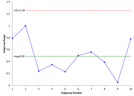
The range chart below in Figure 3 is an example from our article, The Short EMP Study. In this article, an operator measured 10 different parts 3 times each. The range chart is consistent.
Figure 3: Range Chart for Short EMP Study
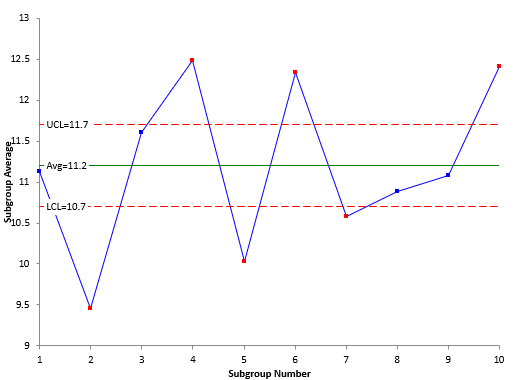
The average range is used in the calculation of the control limits for the X chart. Since the average range represents just measurement error, you want the part averages on the X chart to be out of control as shown in Figure 4. This means that the measurement system can tell the difference between parts in the process. If the parts are representative of the process, you can use that variation to determine the total variance and part variance. If the parts are not representative, you can always use a historical value for the process sigma as shown above in the Consistency Study.
Figure 4: X Chart for Short EMP Study
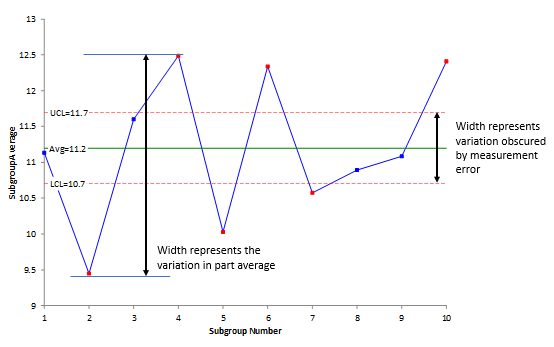
Since the X control limits are based on the measurement error, the width of the control limits represents the amount of part variation that is obscured by the measurement error. This is shown in Figure 5. You cannot see the variation in parts within these control limits because the variation is masked by the measurement error.
Figure 5: Measurement Error Impact on Part Average Variation
Figure 5 also shows the width that is represented by the variation in the average of the parts. You want this width to be greater than the width obscured by the measurement error. This is true in Figure 5. You have indications from this chart that the measurement system can tell the difference between parts most of the time.
If the range chart is consistent, you can begin to do all the characterizations shown in the Consistency Study above. Some of the formulas will be different.
Basic EMP Study
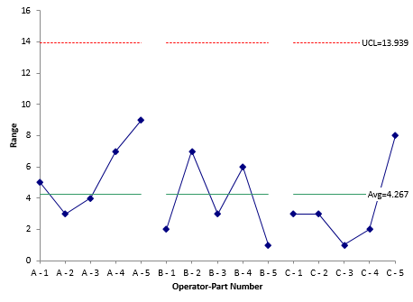
The Basic EMP Study is performed with multiple operators running the same parts multiple times. The results are assessed first by placing them on X–R control chart using the results for one operator and one part to form the subgroups. The R control chart must be in control before you can characterize the measurement system. Again, the range chart represents measurement error.
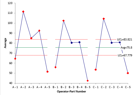
Our article, Evaluating the Measurement Process – Part 2, has an example of the Basic EMP Study. In this example, 3 operators each measure the same 5 parts two times. The X-R control chart (Figures 6 and 7) is shown below.
Figure 6:XChart for the Operator-Part Subgroups
Figure 7: Range Chart for Operator-Part Subgroups
The X chart for the Basic EMP Study is like the X chart for the Short EMP Study – just one for each operator.
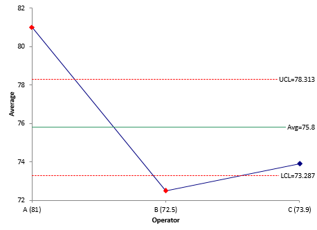
Since there are multiple operators, the analysis also includes an ANOM chart for the main effects (operator averages) to see if there are differences between the operators. Figure 8 below shows that Operator A gets a significantly different average than Operators B and C. You will have to find out why that is the case.
Figure 8: Main Effects Chart
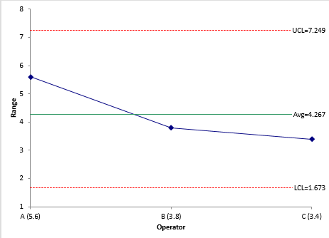
Figure 9 is the mean range chart which compares the average range for each operator. All three operators in this example have the same moving range.
Figure 9: Mean Range Chart
If the range chart and mean range chart are consistent, you can begin to do all the characterizations given in the Consistency Study. Some of the calculations will use different formulas.
Summary
This article has provided an overview to the three major techniques of EMP: the Consistency Study, the Short EMP Study and the Basic EMP Study. The first technique, Consistency Study, involves one operator and one part. The objective is to determine if the measurement system is consistent. If it is not, there is nothing you can really do with it – the measurements are meaningless.
The second technique, the Short EMP Study, involves one operator still but multiple parts. This begins to allow you to determine if the measurement system can tell the difference between parts.
The third technique, the Basic EMP Study, brings additional operators into the study. This allows you to begin to see if differences exist between operators. Regardless of the technique, if the measurement system is consistent, you can begin to characterize the measurement system in many ways as shown in the Consistency Study above.
SPC for Excel Version 6 is Now Available

I received the following comment and have his permission to post it here:
Dear Dr.McNeese, Thank you for your series of presentations titled “SPC for Excel” which I receive. I never miss them. I read them several times. They are very clear, easy to understand and helpful in the practical application. They drive out fear for the application of SPC and encourages those responsible for process control to apply them with clear understanding. With best wishes, Wajira Tirikawala, Senior Member, ASQ